Dask-native OD connectivity with hex_connectivity_dask

This notebook demonstrates how to efficiently compute origin–destination (OD) connectivity from trajectory data using a lazy, dask-backed pipeline. The key benefit: you can filter (e.g., by observation step) before computation to avoid materialising the full trajectory table.

The workflow:

1. Open a dask-backed xarray Dataset (chunked along traj).

2. Build a lazy OD table with hex_connectivity_dask, one row per (traj, obs) pair.

3. Filter to select the target observation step(s).

4. Call .compute() to aggregate and materialise counts.

5. Attach destination hex geometries and visualise.

Setup

import warnings
warnings.filterwarnings("ignore", category=RuntimeWarning)

from importlib.resources import files

import numpy as np
import pandas as pd
import xarray as xr
import dask.dataframe as dd
import geopandas as gpd
import matplotlib.pyplot as plt
import cartopy.io.shapereader as shpreader

from hextraj import HexProj
from hextraj.hex_analysis import hex_connectivity_dask
from hextraj.hex_id import INVALID_HEX_ID

coastlines = gpd.read_file(
    shpreader.natural_earth(resolution="10m", category="physical", name="coastline")
)

Load data

The bundled NW Shelf dataset contains 5 000 Lagrangian particle trajectories advected for 20 observation steps (roughly three weeks) on the NW European Shelf. Dimensions are (traj, obs). Variables lon and lat record particle positions; some positions are NaN (particle became invalid).

Opening with chunks={"traj": 500} produces a dask-backed Dataset — the same pattern used with a Zarr store. Chunking along traj means each partition contains complete trajectories, making isel(obs=...) a cheap in-chunk slice.

p = files("hextraj.data.trajs").joinpath("nwshelf.nc")
ds = xr.open_dataset(p, chunks={"traj": 500})
ds

/var/folders/w1/m9mm9h9167z_gcfzfffr0rgsh6j6kj/T/ipykernel_7036/3848662866.py:2: UserWarning: The specified chunks separate the stored chunks along dimension "traj" starting at index 500. This could degrade performance. Instead, consider rechunking after loading.
  ds = xr.open_dataset(p, chunks={"traj": 500})

<xarray.Dataset> Size: 4MB
Dimensions:      (traj: 5000, obs: 20)
Dimensions without coordinates: traj, obs
Data variables:
    time         (traj, obs) datetime64[ns] 800kB dask.array<chunksize=(500, 20), meta=np.ndarray>
    trajectory   (traj, obs) float64 800kB dask.array<chunksize=(500, 20), meta=np.ndarray>
    lon          (traj, obs) float32 400kB dask.array<chunksize=(500, 20), meta=np.ndarray>
    lat          (traj, obs) float32 400kB dask.array<chunksize=(500, 20), meta=np.ndarray>
    z            (traj, obs) float32 400kB dask.array<chunksize=(500, 20), meta=np.ndarray>
    temperature  (traj, obs) float32 400kB dask.array<chunksize=(500, 20), meta=np.ndarray>
    salinity     (traj, obs) float32 400kB dask.array<chunksize=(500, 20), meta=np.ndarray>
    land         (traj, obs) float32 400kB dask.array<chunksize=(500, 20), meta=np.ndarray>
Attributes:
    feature_type:           trajectory
    Conventions:            CF-1.6/CF-1.7
    ncei_template_version:  NCEI_NetCDF_Trajectory_Template_v2.0
    parcels_version:        2.3.1
    parcels_mesh:           spherical

xarray.Dataset

• Dimensions:
  • traj: 5000
  • obs: 20
• Data variables: (8)
  • time
    (traj, obs)
    datetime64[ns]
    dask.array<chunksize=(500, 20), meta=np.ndarray>

    long_name :

    standard_name :

    time

    axis :

    T

    Array Chunk Bytes 781.25 kiB 78.12 kiB Shape (5000, 20) (500, 20) Dask graph 10 chunks in 2 graph layers Data type datetime64[ns] numpy.ndarray

  • trajectory
    (traj, obs)
    float64
    dask.array<chunksize=(500, 20), meta=np.ndarray>

    long_name :

    Unique identifier for each particle

    cf_role :

    trajectory_id

    Array Chunk Bytes 781.25 kiB 78.12 kiB Shape (5000, 20) (500, 20) Dask graph 10 chunks in 2 graph layers Data type float64 numpy.ndarray

  • lon
    (traj, obs)
    float32
    dask.array<chunksize=(500, 20), meta=np.ndarray>

    long_name :

    standard_name :

    longitude

    units :

    degrees_east

    axis :

    X

    Array Chunk Bytes 390.62 kiB 39.06 kiB Shape (5000, 20) (500, 20) Dask graph 10 chunks in 2 graph layers Data type float32 numpy.ndarray

  • lat
    (traj, obs)
    float32
    dask.array<chunksize=(500, 20), meta=np.ndarray>

    long_name :

    standard_name :

    latitude

    units :

    degrees_north

    axis :

    Y

    Array Chunk Bytes 390.62 kiB 39.06 kiB Shape (5000, 20) (500, 20) Dask graph 10 chunks in 2 graph layers Data type float32 numpy.ndarray

  • z
    (traj, obs)
    float32
    dask.array<chunksize=(500, 20), meta=np.ndarray>

    long_name :

    standard_name :

    depth

    units :

    m

    positive :

    down

    Array Chunk Bytes 390.62 kiB 39.06 kiB Shape (5000, 20) (500, 20) Dask graph 10 chunks in 2 graph layers Data type float32 numpy.ndarray

  • temperature
    (traj, obs)
    float32
    dask.array<chunksize=(500, 20), meta=np.ndarray>

    long_name :

    standard_name :

    temperature

    units :

    unknown

    Array Chunk Bytes 390.62 kiB 39.06 kiB Shape (5000, 20) (500, 20) Dask graph 10 chunks in 2 graph layers Data type float32 numpy.ndarray

  • salinity
    (traj, obs)
    float32
    dask.array<chunksize=(500, 20), meta=np.ndarray>

    long_name :

    standard_name :

    salinity

    units :

    unknown

    Array Chunk Bytes 390.62 kiB 39.06 kiB Shape (5000, 20) (500, 20) Dask graph 10 chunks in 2 graph layers Data type float32 numpy.ndarray

  • land
    (traj, obs)
    float32
    dask.array<chunksize=(500, 20), meta=np.ndarray>

    long_name :

    standard_name :

    land

    units :

    unknown

    Array Chunk Bytes 390.62 kiB 39.06 kiB Shape (5000, 20) (500, 20) Dask graph 10 chunks in 2 graph layers Data type float32 numpy.ndarray

• Attributes: (5)

  feature_type :

  trajectory

  Conventions :

  CF-1.6/CF-1.7

  ncei_template_version :

  NCEI_NetCDF_Trajectory_Template_v2.0

  parcels_version :

  2.3.1

  parcels_mesh :

  spherical

Build HexProj

A Lambert Azimuthal Equal-Area projection centred near the NW Shelf domain midpoint (−3°E, 54°N) minimises distortion across the region. A hex size of 40 km gives a fine spatial resolution — each hexagon covers roughly 4 200 km², comparable to a 65 × 65 km grid cell.

hp = HexProj(
    projection_name="laea",
    lon_origin=-3.0,
    lat_origin=54.0,
    hex_size_meters=40_000,
    hex_orientation="flat",
)
hp

HexProj(projection_name='laea', lon_origin=-3.0, lat_origin=54.0, hex_size_meters=40000, hex_orientation='flat', )

Build the lazy connectivity table

hex_connectivity_dask builds a lazy dask DataFrame with one row per (traj, obs) combination. No computation happens here — the function wires together the dask task graph without reading any data.

The result always contains:

Column	Description
from_id	hex ID at obs=0 for each trajectory (the release hex)
to_id	hex ID at the current obs step
obs	observation index (0 … 19)
traj	trajectory index

INVALID_HEX_ID = -1 appears in from_id or to_id wherever the particle position is NaN (became invalid early and is absent from subsequent analysis).

ddf = hex_connectivity_dask(ds, hp)
ddf

Dask DataFrame Structure:

	traj	obs	to_id	from_id
npartitions=10
0	int64	int64	int64	int64
10000	...	...	...	...
...	...	...	...	...
90000	...	...	...	...
99999	...	...	...	...

Dask Name: label, 10 expressions

Understanding laziness

A dask DataFrame is lazy: the function constructs a task graph describing the computation without reading any data or executing it. You control when execution happens — by calling .compute() — and you can filter the graph before that point (e.g., select only one observation step) to avoid materialising the full table.

We can inspect the size of the task graph to verify the pipeline is fully encoded:

print(f"Number of tasks in the dask graph: {len(ddf.__dask_graph__())}")
print(f"Number of partitions: {ddf.npartitions}")

Number of tasks in the dask graph: 187
Number of partitions: 10

Filter before compute

The user decides what to aggregate before calling .compute(). Here we select only rows where obs equals the final observation step (obs=19). This reduces the materialised data from the full (traj × obs) table to just the last observation per trajectory — without triggering any I/O.

last_obs = int(ds["obs"].values[-1])
ddf_last = ddf[ddf["obs"] == last_obs]
print(f"After filter: {type(ddf_last).__name__} with obs={last_obs}")

After filter: DataFrame with obs=19

Compute obs=0 → obs=19 connectivity

Now we materialise: group by (from_id, to_id), count trajectories per pair, then drop rows involving INVALID_HEX_ID (particles that left the domain at either the start or end of their trajectory).

The single .compute() call executes the full pipeline: read chunks from disk, project lon/lat to hex IDs, filter, and aggregate.

od = (
    ddf_last
    .groupby(["from_id", "to_id"])
    .size()
    .compute()
)
od.name = "count"

od = od[
    (od.index.get_level_values("from_id") != INVALID_HEX_ID)
    & (od.index.get_level_values("to_id") != INVALID_HEX_ID)
]

Top-10 OD pairs

Pairs where from_id == to_id represent trajectories that stayed in the same hex from release to the final step — these dominate the ranking and indicate strong retention in their release hexagons.

od.nlargest(10).to_frame()

		count
from_id	to_id
80	80	12
112	145	12
174	174	12
391	391	12
69	125	11
59	59	11
85	85	10
143	180	10
140	140	10
266	266	10

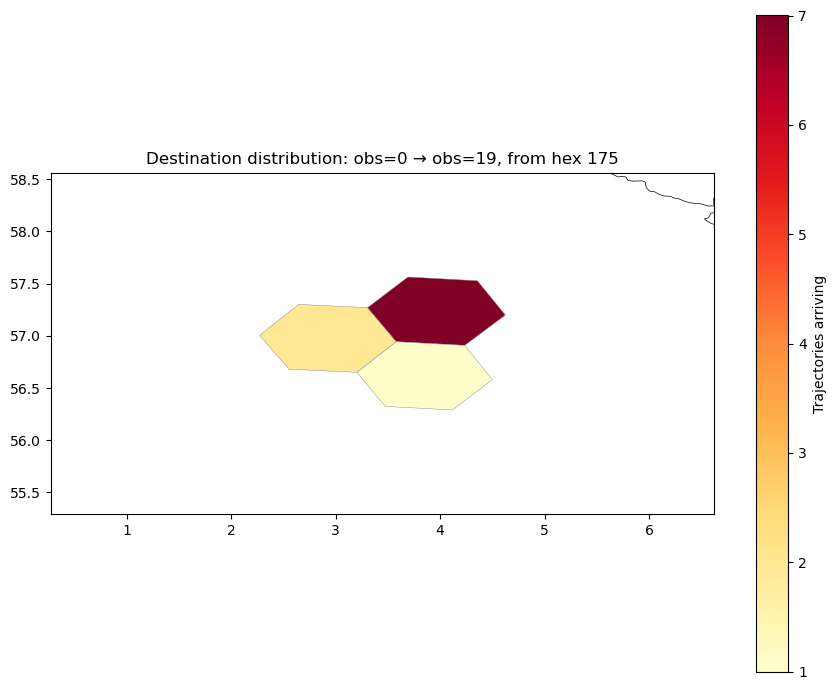
Visualise as a choropleth heatmap

The plots below show connectivity from a fixed origin hex in the central North Sea (~4°E, 57°N). This location sits in the open northern North Sea, away from coastal boundaries, giving a clean picture of offshore dispersal driven by the large-scale circulation. With 40 km hexes, the origin region is well-resolved and contains enough trajectories for statistically meaningful destination maps.

hp.to_geodataframe accepts an array of hex IDs and returns a GeoDataFrame with hexagonal Polygon geometries in EPSG:4326.

from_hex = 175  # central North Sea, ~4°E 57°N (200 trajectories)

dest = od.xs(from_hex, level="from_id")
dest = dest[dest.index != INVALID_HEX_ID]
dest_ids = dest.index.values

dest_gdf = hp.to_geodataframe(dest_ids, count=dest.values)
dest_gdf = dest_gdf[dest_gdf.geometry.notna()]
dest_gdf.head()

	count	geometry
140	2	POLYGON ((3.58046 56.94363, 3.20205 56.6502, 2...
175	7	POLYGON ((4.62351 57.19864, 4.23426 56.90838, ...
138	1	POLYGON ((4.49912 56.58035, 4.11742 56.28969, ...

fig, ax = plt.subplots(figsize=(9, 7))

dest_gdf.plot(
    column="count",
    ax=ax,
    cmap="YlOrRd",
    edgecolor="grey",
    linewidth=0.3,
    legend=True,
    legend_kwds={"label": "Trajectories arriving", "orientation": "vertical"},
)
coastlines.plot(ax=ax, color="black", linewidth=0.5)

bounds = dest_gdf.total_bounds
ax.set_xlim(bounds[0] - 2, bounds[2] + 2)
ax.set_ylim(bounds[1] - 1, bounds[3] + 1)
ax.set_title(f"Destination distribution: obs=0 → obs=19, from hex {from_hex}")
plt.tight_layout()
plt.show()

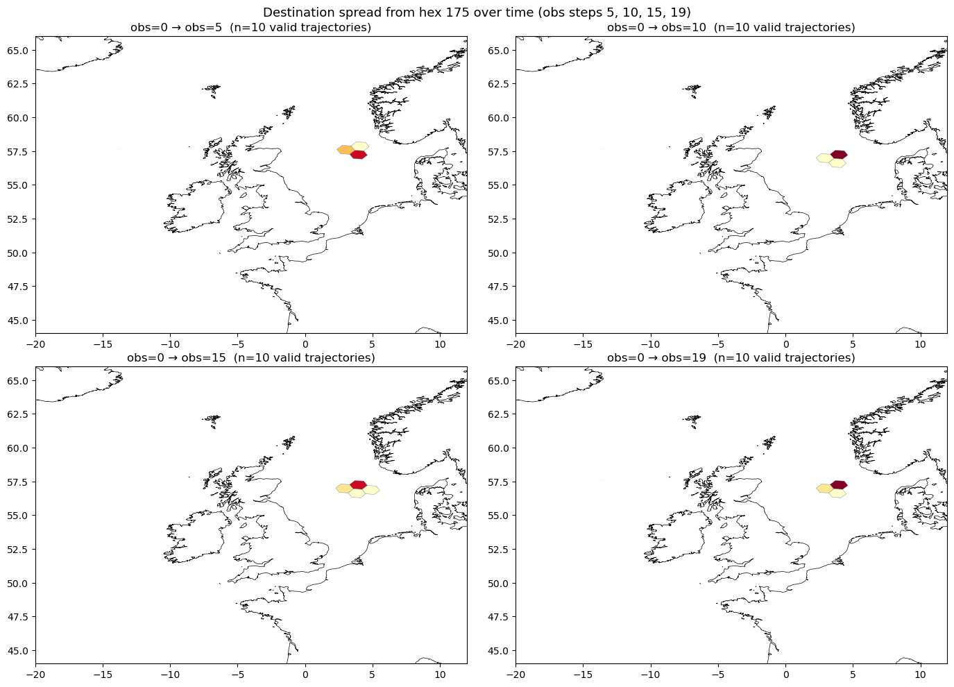
Multi-obs view: spreading over time

Applying the same connectivity analysis at multiple observation steps shows how trajectories spread spatially over time. By filtering to each step before computing, we avoid materialising the entire lazy DataFrame — the filter predicate is added to the task graph before execution.

obs_steps = [5, 10, 15, 19]

od_by_obs = {}
for k in obs_steps:
    od_k = (
        ddf[ddf["obs"] == k]
        .groupby(["from_id", "to_id"])
        .size()
        .compute()
    )
    od_k.name = "count"
    od_k = od_k[
        (od_k.index.get_level_values("from_id") != INVALID_HEX_ID)
        & (od_k.index.get_level_values("to_id") != INVALID_HEX_ID)
    ]
    od_by_obs[k] = od_k

print("Computed OD counts at obs steps:", list(od_by_obs.keys()))

Computed OD counts at obs steps: [5, 10, 15, 19]

fig, axes = plt.subplots(2, 2, figsize=(14, 10))

for ax, k in zip(axes.flat, obs_steps):
    od_k = od_by_obs[k]

    try:
        dest_k = od_k.xs(from_hex, level="from_id")
    except KeyError:
        dest_k = pd.Series(dtype=int, name="count")

    dest_k = dest_k[dest_k.index != INVALID_HEX_ID]

    if len(dest_k) > 0:
        dest_k_gdf = hp.to_geodataframe(dest_k.index.values, count=dest_k.values)
        dest_k_gdf = dest_k_gdf[dest_k_gdf.geometry.notna()]

        dest_k_gdf.plot(
            column="count",
            ax=ax,
            cmap="YlOrRd",
            edgecolor="grey",
            linewidth=0.3,
            vmin=1,
            vmax=od.xs(from_hex, level="from_id").max(),
            legend=False,
        )

    coastlines.plot(ax=ax, color="black", linewidth=0.5)

    n_traj = int(dest_k.sum()) if len(dest_k) > 0 else 0
    ax.set_xlim(-20, 12)
    ax.set_ylim(44, 66)
    ax.set_title(f"obs=0 → obs={k}  (n={n_traj} valid trajectories)")

fig.suptitle(
    f"Destination spread from hex {from_hex} over time (obs steps 5, 10, 15, 19)",
    fontsize=13,
)
plt.tight_layout()
plt.show()

Cumulative settling connectivity

A particle that can settle — recruit to a habitat, land on the seabed — performs this action exactly once, at the first step where the condition is met. If the probability of settling is equal at every observation step, then the probability of settling in hex $j$ is proportional to the total time spent in hex $j$.

For a particle released in hex $i$, let $n_{ij}$ be the total number of (traj, obs) pairs for which from_id = $i$ and to_id = $j$ — i.e., the cumulative visits to hex $j$ across all obs steps. The settling probability is:

$$P(\text{settles in } j \mid \text{released in } i) = \frac{n_{ij}}{\displaystyle\sum_{j’} n_{ij’}}$$

No weight column is needed: equal-probability settling reduces to counting visits.

This contrasts with the endpoint view (obs=0 → obs=19), which records only where each particle ends up at the final step. Particles that pass through a hex early and then leave contribute nothing to the endpoint count, even if they would have settled there with high probability. The settling view integrates over the entire trajectory.

Compute settling connectivity

Group by (from_id, to_id) across all observation steps and count rows. The full lazy DataFrame ddf is used — no pre-filtering by obs step.

settling = (
    ddf.groupby(["from_id", "to_id"])
    .size()
    .compute()
    .rename("settling_probability")
)

Normalise per origin hex

Dividing by the total visit count out of each origin converts raw counts into conditional probabilities: the fraction of visits to hex $j$ among all visits from origin $i$. Each row of the resulting table sums to 1 over all valid destinations.

settling_norm = settling / settling.groupby(level="from_id").transform("sum")

Compare endpoint vs. settling connectivity

Two panels for the same origin hex from_hex:

• Left: endpoint connectivity — only trajectories that reach obs=19, showing where particles end up at the final step.

• Right: settling connectivity — the time-averaged fraction of visits to each hex, integrating over all obs steps.

A hex that particles pass through early and leave will appear in the right panel but not in the left. Conversely, hexes that particles drift into only near the end will dominate the left panel.

try:
    dest_endpoint = od.xs(from_hex, level="from_id")
except KeyError:
    dest_endpoint = pd.Series(dtype=float, name="count")

dest_endpoint = dest_endpoint[dest_endpoint.index != INVALID_HEX_ID]
dest_endpoint_norm = dest_endpoint / dest_endpoint.sum()

try:
    dest_settling = settling_norm.xs(from_hex, level="from_id")
except KeyError:
    dest_settling = pd.Series(dtype=float, name="settling_probability")

dest_settling = dest_settling[dest_settling.index != INVALID_HEX_ID]

all_ids = np.union1d(dest_endpoint_norm.index.values, dest_settling.index.values)
vmax = max(dest_endpoint_norm.max(), dest_settling.max())

fig, axes = plt.subplots(1, 2, figsize=(16, 7))

for ax, values, title in zip(
    axes,
    [dest_endpoint_norm, dest_settling],
    [
        f"Endpoint connectivity\nobs=0 → obs=19, from hex {from_hex}",
        f"Settling connectivity (time-averaged)\nall obs steps, from hex {from_hex}",
    ],
):
    ids = values.index.values
    if len(ids) > 0:
        gdf = hp.to_geodataframe(ids, value=values.values)
        gdf = gdf[gdf.geometry.notna()]
        gdf.plot(
            column="value",
            ax=ax,
            cmap="YlOrRd",
            edgecolor="grey",
            linewidth=0.3,
            vmin=0,
            vmax=vmax,
            legend=True,
            legend_kwds={"label": "Probability", "orientation": "vertical"},
        )
    coastlines.plot(ax=ax, color="black", linewidth=0.5)
    ax.set_xlim(-20, 12)
    ax.set_ylim(44, 66)
    ax.set_title(title)

plt.tight_layout()
plt.show()

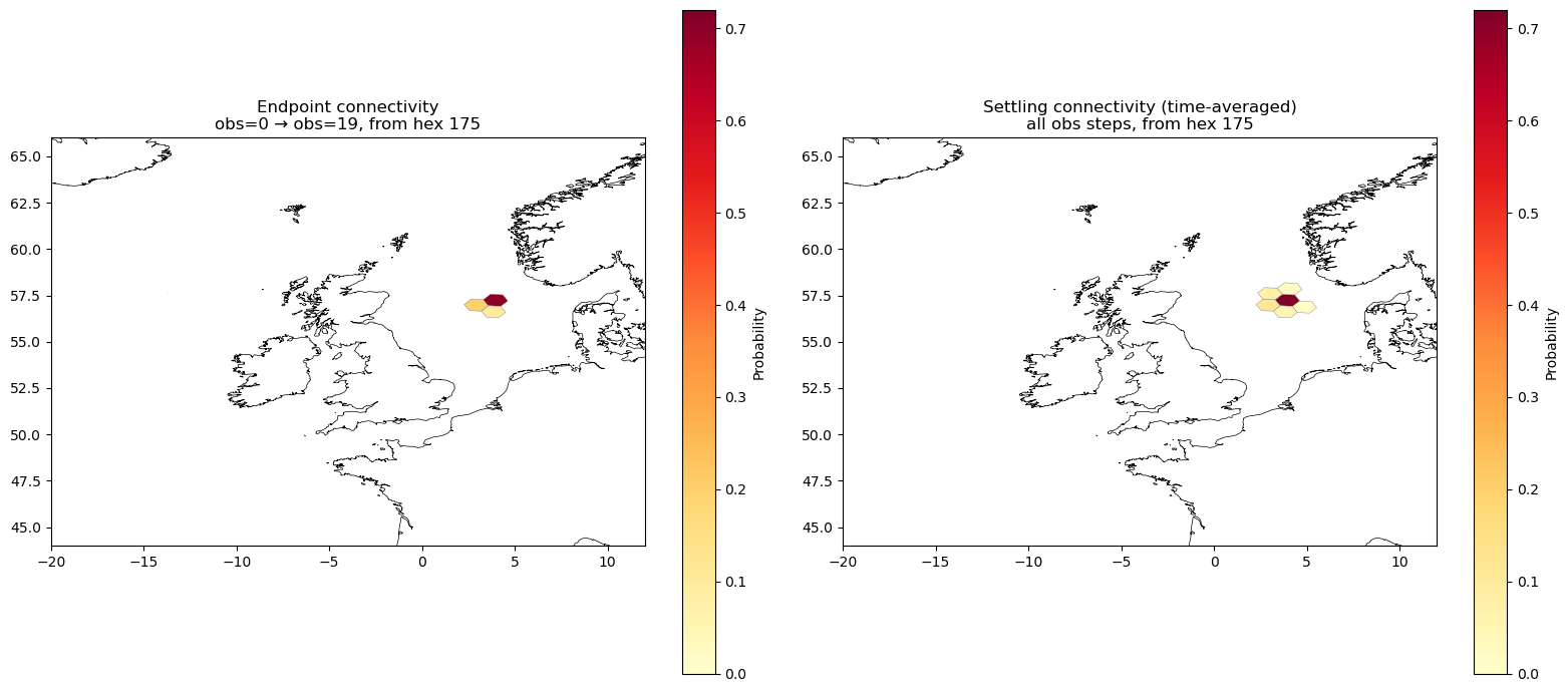
Interpretation

The two panels show different aspects of the same trajectories. In the left panel, only particles still valid at obs=19 contribute — particles that became invalid early are absent from the count. The spatial pattern reflects where particles happen to be at one particular moment.

The right panel accumulates visits across all 20 obs steps. A hex that particles cross through at any point — even obs=1 — contributes to its settling probability. Hexes close to the release point often receive more probability mass in the settling view because particles spend more total time near their origin than they do near any single distant destination. Conversely, distant hexes that particles reach only late in the simulation may appear equally prominent in the endpoint panel but weaker in the settling panel, because particles spent fewer steps there overall.

The settling view is the physically appropriate connectivity metric when the action of interest — recruitment, deposition, colonisation — can happen at any step with equal likelihood. The endpoint view is appropriate only when the relevant moment is fixed (e.g. arrival at a sampling date).