Trajectory → hex aggregation → choropleth

This notebook demonstrates the complete pipeline from raw positional data to a choropleth map:

1. Set up a HexProj instance covering the North Sea.

2. Generate synthetic trajectory positions scattered over the region.

3. Assign a hex ID to every position with hp.label().

4. Count visits per hex with a pandas value_counts().

5. Build the full hex universe for the region polygon.

6. Join counts onto that universe so unvisited hexes show zero.

7. Plot the result as a choropleth with a coastline overlay.

Imports

from hextraj import HexProj

import numpy as np
import pandas as pd
import geopandas as gpd
from shapely.geometry import Polygon
from matplotlib import pyplot as plt

Projection setup

We use Lambert Azimuthal Equal-Area centred on the North Sea (10 °E, 55 °N) with 20 km hexes — fine enough to resolve individual shipping lanes.

hp = HexProj(
    projection_name="laea",
    lon_origin=10,
    lat_origin=55,
    hex_size_meters=20_000,
)
hp

HexProj(projection_name='laea', lon_origin=10, lat_origin=55, hex_size_meters=20000, hex_orientation='flat', )

Synthetic ship tracks

We generate 10 synthetic vessel trajectories that follow realistic North Sea routes — Dover Strait to the Norwegian coast, Rotterdam to Aberdeen, English Channel to Skagerrak, and similar corridors. Each track is a straight-line great-circle route between two waypoints with small random-walk noise added at every step (std ≈ 0.05–0.1 °) to mimic realistic GPS traces. All tracks are concatenated into a single lon/lat array.

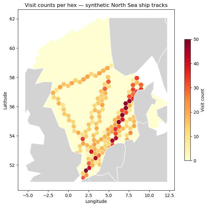
When aggregated onto the hex grid, this produces high visit counts along the main shipping lanes and near-zero counts elsewhere — much closer to real AIS density patterns than a Gaussian blob.

rng = np.random.default_rng(seed=42)

# Realistic North Sea routes: (lon_start, lat_start, lon_end, lat_end, n_steps, noise_std)
routes = [
    ( 2.0, 51.1,  5.0, 58.0, 400, 0.06),   # Dover Strait → Norwegian coast
    ( 4.2, 51.9, -2.1, 57.1, 350, 0.07),   # Rotterdam → Aberdeen
    ( 1.5, 51.0,  9.8, 57.5, 450, 0.08),   # English Channel → Skagerrak
    ( 5.3, 53.1,  8.7, 58.3, 300, 0.05),   # IJmuiden → Bergen
    ( 0.1, 51.4,  4.9, 57.9, 380, 0.07),   # Thames estuary → Stavanger
    (-1.6, 57.2,  5.5, 58.6, 250, 0.06),   # Aberdeen → Stavanger
    ( 7.0, 53.3, 10.5, 57.8, 320, 0.05),   # Bremerhaven → Göteborg
    ( 4.5, 52.0,  8.8, 58.2, 360, 0.08),   # Rotterdam → Bergen
    ( 1.8, 51.2,  8.1, 55.5, 280, 0.06),   # Dover → Danish coast
    ( 3.0, 53.0, 10.0, 58.5, 420, 0.09),   # North Sea crossing (central)
]

track_lons, track_lats = [], []

for lon0, lat0, lon1, lat1, n, noise_std in routes:
    t = np.linspace(0, 1, n)
    lons = lon0 + (lon1 - lon0) * t + rng.normal(0, noise_std, size=n).cumsum() * 0.1
    lats = lat0 + (lat1 - lat0) * t + rng.normal(0, noise_std, size=n).cumsum() * 0.1
    track_lons.append(lons)
    track_lats.append(lats)

lon = np.concatenate(track_lons)
lat = np.concatenate(track_lats)
print(f"{len(lon):,} positions across {len(routes)} ship tracks")

3,510 positions across 10 ship tracks

Label positions

hp.label() maps every (lon, lat) pair to a single int64 hex ID.

hex_ids = hp.label(lon, lat)
print(f"Unique hexes visited: {len(np.unique(hex_ids))}")

Unique hexes visited: 196

Aggregate — count visits per hex

pd.Series.value_counts() gives us the number of positions that fell inside each hex ID.

counts = pd.Series(hex_ids).value_counts()
counts.head()

667    50
286    49
284    48
288    48
339    48
Name: count, dtype: int64

Build the full hex universe for the region

We use the same rough North Sea polygon as in hex_grid_construction.ipynb. region_of_hexes returns every hex whose polygon intersects the region; to_geodataframe converts those IDs to a GeoDataFrame with hex polygons in EPSG:4326.

The synthetic tracks only pass through a subset of hexes — including the full regional universe means route-free hexes appear in the lightest colour rather than being absent from the map.

north_sea = Polygon([
    (-5,  57),
    ( 2,  51),
    ( 9,  53),
    (12,  56),
    ( 8,  58),
    ( 5,  62),
    (-3,  60),
    (-5,  57),
])

region_gdf = hp.to_geodataframe(hp.region_of_hexes(north_sea))
print(f"{len(region_gdf)} hexes in North Sea region")
region_gdf.head()

772 hexes in North Sea region

	geometry
5611	POLYGON ((-4.46675 56.66501, -4.56734 56.49466...
5826	POLYGON ((-4.58574 56.96852, -4.68643 56.79807...
6045	POLYGON ((-4.70701 57.27188, -4.80778 57.10134...
4793	POLYGON ((-3.70733 55.9591, -3.80979 55.78933,...
4992	POLYGON ((-3.81737 56.26343, -3.91998 56.09358...

Join counts onto the hex universe

We reindex the visit counts against the full set of regional hex IDs and fill missing values with zero. This left-join pattern ensures that hexes with no visits appear as 0 rather than NaN, which keeps the colour scale honest.

region_gdf["count"] = counts.reindex(region_gdf.index).fillna(0).astype(int)
region_gdf[["count"]].describe()

	count
count	772.000000
mean	4.338083
std	9.258274
min	0.000000
25%	0.000000
50%	0.000000
75%	0.000000
max	50.000000

Plot choropleth

Each hex is coloured by its visit count using a sequential colour map (yellow → red). Coastlines from Natural Earth (same URL as in hex_grid_construction.ipynb) are overlaid for geographic context. Hexes with zero visits appear in the lightest yellow, making the density gradient immediately legible.

world = gpd.read_file(
    "https://naciscdn.org/naturalearth/110m/cultural/ne_110m_admin_0_countries.zip"
)

ax = region_gdf.plot(
    column="count",
    cmap="YlOrRd",
    edgecolor="white",
    linewidth=0.6,
    figsize=(7, 7),
    legend=True,
    legend_kwds={"label": "Visit count", "shrink": 0.6},
)
world.clip(region_gdf.total_bounds).plot(ax=ax, color="lightgray", edgecolor="white")
ax.set_title("Visit counts per hex — synthetic North Sea ship tracks")
ax.set_xlabel("Longitude")
ax.set_ylabel("Latitude")
plt.tight_layout()

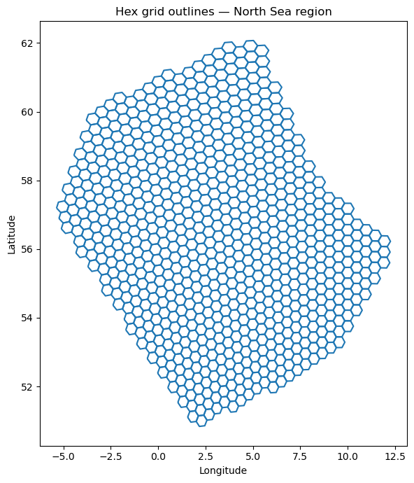
Hex outlines

The boundary of each hex polygon can be extracted as a LineString using .boundary. This view emphasises the grid structure itself — useful for checking projection accuracy or understanding the grid’s geometric properties.

ax = region_gdf.boundary.plot(figsize=(7, 7))
ax.set_title("Hex grid outlines — North Sea region")
ax.set_xlabel("Longitude")
ax.set_ylabel("Latitude")
plt.tight_layout()

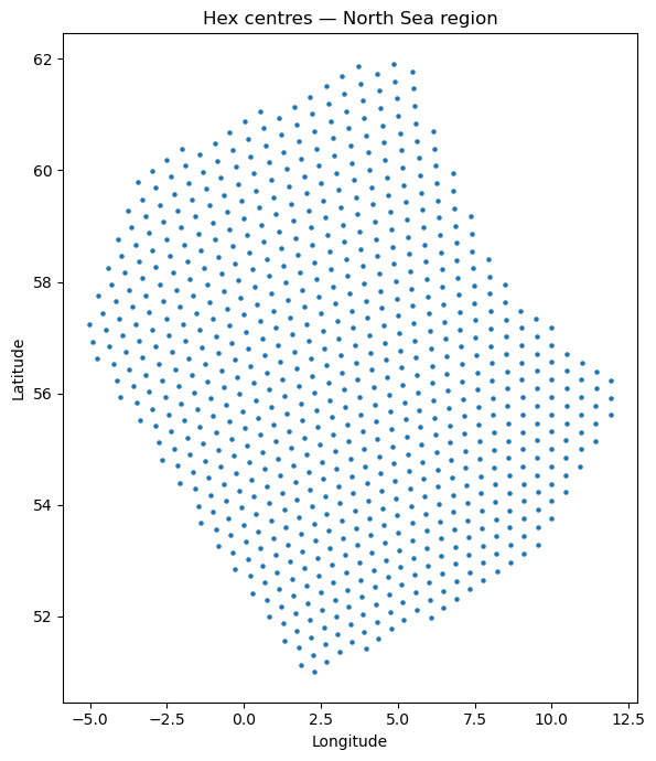
Hex centers

The centroid of each hex polygon lies at its centre. Switching the active geometry to centroids with .set_geometry(gdf.centroid) plots the grid as discrete points instead of filled polygons.

ax = region_gdf.set_geometry(region_gdf.centroid).plot(
    markersize=5,
    figsize=(7, 7),
)
ax.set_title("Hex centres — North Sea region")
ax.set_xlabel("Longitude")
ax.set_ylabel("Latitude")
plt.tight_layout()

/var/folders/w1/m9mm9h9167z_gcfzfffr0rgsh6j6kj/T/ipykernel_7003/1382084793.py:1: UserWarning: Geometry is in a geographic CRS. Results from 'centroid' are likely incorrect. Use 'GeoSeries.to_crs()' to re-project geometries to a projected CRS before this operation.

  ax = region_gdf.set_geometry(region_gdf.centroid).plot(

Origin–destination edges

Each ship route connects a fixed origin port to a fixed destination port. Labelling those two endpoints with hp.label() gives one hex ID pair per journey. When the same route is taken multiple times, grouping by (origin, destination) and counting gives a weighted OD matrix — one edge per unique route, weight = number of journeys.

origin_lons = np.array([r[0] for r in routes])
origin_lats = np.array([r[1] for r in routes])
dest_lons   = np.array([r[2] for r in routes])
dest_lats   = np.array([r[3] for r in routes])

origin_hexes = hp.label(origin_lons, origin_lats)
dest_hexes   = hp.label(dest_lons,   dest_lats)
print(f"{len(routes)} routes → {len(set(zip(origin_hexes, dest_hexes)))} unique OD pairs")

10 routes → 10 unique OD pairs

od_gdf = hp.edges_geodataframe(
    origin_hexes,
    dest_hexes,
    weight=np.ones(len(routes), dtype=int),
)
print(f"OD edges: {od_gdf.shape}")
od_gdf

OD edges: (10, 2)

		weight	geometry
from_id	to_id
823	1255	1	LINESTRING (1.84222 51.12476, 4.92177 58.01285)
470	4047	1	LINESTRING (4.32862 51.90227, -1.98905 57.24142)
906	152	1	LINESTRING (1.44561 50.93848, 10 57.48914)
211	459	1	LINESTRING (5.5238 53.04701, 8.46753 58.25808)
1130	1255	1	LINESTRING (0.07581 51.29617, 4.92177 58.01285)
3695	1257	1	LINESTRING (-1.45059 57.13353, 5.36821 58.49713)
139	228	1	LINESTRING (6.85325 53.24612, 10.5065 57.95487)
470	347	1	LINESTRING (4.32862 51.90227, 8.98268 58.10748)
823	128	1	LINESTRING (1.84222 51.12476, 8.09573 55.60765)
634	275	1	LINESTRING (2.85187 52.91381, 10 58.42258)

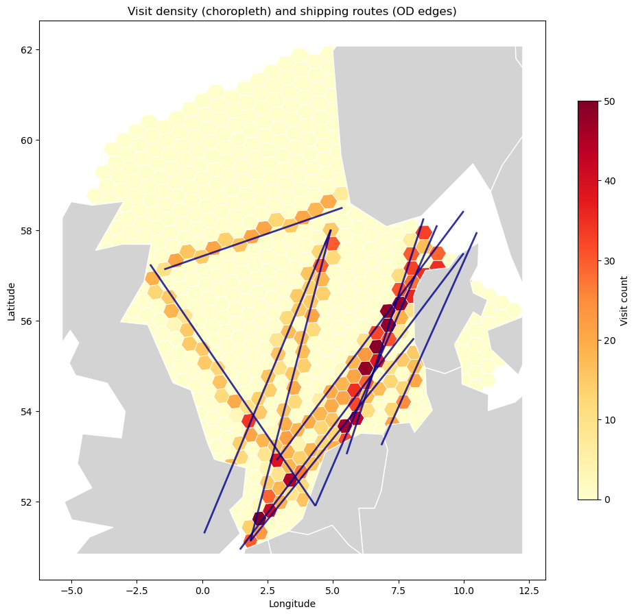
Combined plot: choropleth with OD edges overlay

The choropleth shows visit density from the full trajectories. The OD edges connect origin and destination hex centres with straight lines — each line is one shipping route. This view separates the flow topology (where ships go) from the spatial density (where ships spend time).

ax = region_gdf.plot(
    column="count",
    cmap="YlOrRd",
    edgecolor="white",
    linewidth=0.6,
    figsize=(10, 10),
    legend=True,
    legend_kwds={"label": "Visit count", "shrink": 0.6},
)
world.clip(region_gdf.total_bounds).plot(ax=ax, color="lightgray", edgecolor="white")

od_gdf.plot(ax=ax, linewidth=2, color="darkblue", alpha=0.8)

ax.set_title("Visit density (choropleth) and shipping routes (OD edges)")
ax.set_xlabel("Longitude")
ax.set_ylabel("Latitude")
plt.tight_layout()