Hex Analysis: Heatmaps and Connectivity#

This notebook demonstrates two analysis functions from hextraj:

hex_counts — aggregate trajectory observations into a spatial heatmap, counting how many times each hex cell was visited across a dataset.
hex_connectivity — build a start-to-end connectivity matrix that records how many trajectories travelled from each origin hex to each destination hex.

Both functions operate on xr.DataArray objects of integer hex IDs produced by HexProj.label(). They return GeoDataFrame objects, which carry geometry alongside statistics and integrate directly with geopandas and matplotlib for visualisation.

The dataset used here is the bundled NW European Shelf trajectory dataset: 5 000 Lagrangian particles advected for 20 observations (roughly three weeks) in May–June 2019.

Setup#

import numpy as np
import xarray as xr
import geopandas as gpd
import matplotlib.pyplot as plt
import matplotlib.cm as cm
import matplotlib.colors as mcolors
import cartopy.io.shapereader as shpreader
from importlib.resources import files

from hextraj import HexProj, hex_counts, hex_connectivity
from hextraj.hex_id import INVALID_HEX_ID

coastlines = gpd.read_file(
    shpreader.natural_earth(resolution="10m", category="physical", name="coastline")
)

Build a HexProj for the NW Shelf domain#

The NW Shelf domain spans roughly 46–63 °N and 16 °W–10 °E. A Lambert Azimuthal Equal-Area projection centred near the domain midpoint (−3 °E, 54 °N) minimises distortion across the region.

A hex size of 100 km (corner-to-centre distance) gives a coarse but meaningful spatial resolution — each hexagon covers roughly 26 000 km². Larger sizes produce a sparser grid with higher counts per cell; smaller sizes resolve more spatial detail but require more data to populate.

hp = HexProj(
    projection_name="laea",
    lon_origin=-3.0,
    lat_origin=54.0,
    hex_size_meters=100_000,
    hex_orientation="flat",
)
hp

HexProj(projection_name='laea', lon_origin=-3.0, lat_origin=54.0, hex_size_meters=100000, hex_orientation='flat', )

Label every (traj, obs) position with its hex ID. NaN positions (particles that have left the domain) are assigned INVALID_HEX_ID = -1 by hp.label().

hex_ids = xr.DataArray(
    hp.label(ds.lon.values, ds.lat.values),
    dims=["traj", "obs"],
)
hex_ids

<xarray.DataArray (traj: 5000, obs: 20)> Size: 800kB
array([[245, 245, 245, ..., 245, 245, 245],
       [ 20,  20,  20, ...,  20,  20,  20],
       [126, 126, 126, ...,  97,  97,  97],
       ...,
       [ 48,  48,  48, ...,  48,  48,  48],
       [ 29,  29,  29, ...,  29,  29,  29],
       [ 76,  76,  76, ...,  76,  76,  76]], shape=(5000, 20))
Dimensions without coordinates: traj, obs

Hex heatmap: `hex_counts`#

hex_counts answers the question: how many trajectory observations fell in each hex cell, summing over a chosen set of dimensions?

Formally, let $\mathbf{H}$ be the hex ID tensor indexed by $(k, r)$ where $k$ are “keep” indices and $r$ are “reduce” indices. Define the indicator

$$X_h(k, r) = \begin{cases} 1 & \text{if } H(k,r) = h \ 0 & \text{otherwise,} \end{cases}$$

then the count for hex $h$ at keep-index $k$ is

$$C(k, h) = \sum_{r \in \mathcal{R}} X_h(k, r).$$

The result is a GeoDataFrame indexed by hex_id, with columns count and geometry (a hexagonal polygon in EPSG:4326). Hex IDs that were never observed are absent. The special bucket INVALID_HEX_ID = -1 captures all out-of-domain positions and is included in the result with geometry = None.

Reduce over both traj and obs to get the total visit count per hex across all trajectories and all time steps.

counts = hex_counts(hex_ids, reduce_dims=["traj", "obs"], hp=hp)
counts

	count	geometry
hex_id
-1	2915	None
0	423	POLYGON ((-1.47527 53.99035, -2.25145 53.21952...
1	985	POLYGON ((-3.74855 53.21952, -4.47037 52.43438...
3	802	POLYGON ((0.88138 54.71646, 0.04815 53.96142, ...
4	874	POLYGON ((-3.72252 51.66296, -4.42048 50.87772...
...	...	...
243	507	POLYGON ((-14.34503 58.9706, -14.93841 58.1302...
245	1211	POLYGON ((-12.39371 61.47694, -13.07512 60.644...
290	213	POLYGON ((-14.87452 60.50265, -15.47743 59.659...
292	619	POLYGON ((-12.88008 63.0179, -13.57864 62.182,...
341	11	POLYGON ((-15.46368 62.03277, -16.07536 61.186...

117 rows × 2 columns

The INVALID_HEX_ID row (index value −1) has geometry = None and records the total number of observations where the particle had left the domain. Inspect it separately, then drop it before plotting.

print("INVALID_HEX_ID row:")
print(counts.loc[INVALID_HEX_ID])
print()
print(f"Out-of-domain observations: {counts.loc[INVALID_HEX_ID, 'count']}")
print(f"Total observations: {counts['count'].sum()}")

INVALID_HEX_ID row:
count       2915
geometry    None
Name: -1, dtype: object

Out-of-domain observations: 2915
Total observations: 100000

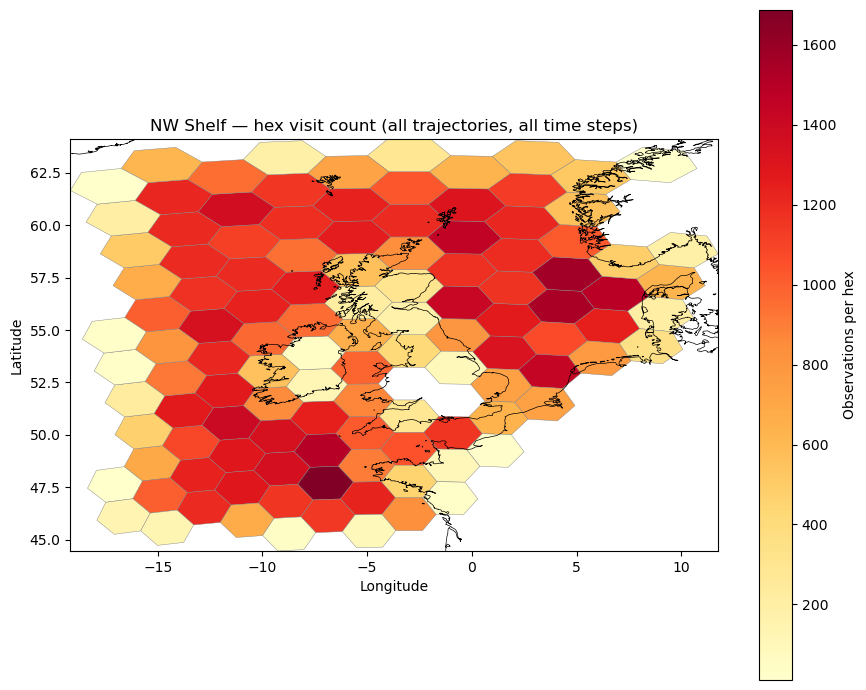
Drop the invalid row and plot the heatmap. Each polygon is coloured by its total visit count.

counts_valid = counts.drop(index=INVALID_HEX_ID, errors="ignore")

fig, ax = plt.subplots(figsize=(9, 7))
counts_valid.plot(
    column="count",
    ax=ax,
    legend=True,
    legend_kwds={"label": "Observations per hex", "orientation": "vertical"},
    cmap="YlOrRd",
    edgecolor="grey",
    linewidth=0.3,
)
coastlines.plot(ax=ax, color="black", linewidth=0.5)
ax.set_xlim(counts_valid.total_bounds[[0, 2]])
ax.set_ylim(counts_valid.total_bounds[[1, 3]])
ax.set_title("NW Shelf — hex visit count (all trajectories, all time steps)")
ax.set_xlabel("Longitude")
ax.set_ylabel("Latitude")
plt.tight_layout()
plt.show()

../_images/e0650850a85c68a9414af84f8980658a0149a3a6b8ecc1f185a330a30e756646.png

Connectivity: `hex_connectivity`#

hex_connectivity answers the question: how many trajectories started in hex $h_0$ and ended in hex $h_1$?

Select the release position with from_dim="obs", from_idx=0 and the final position with to_dim="obs", to_idx=-1. For each trajectory the function extracts a (start hex, end hex) pair and counts how many trajectories share each unique pair:

$$C(h_0, h_1) = \text{count}\bigl(\text{start} = h_0,\ \text{end} = h_1\bigr).$$

The result is a GeoDataFrame with a (from_id, to_id) MultiIndex and a count column. Trajectories that exit the simulation domain arrive at INVALID_HEX_ID = -1 as their destination — these pairs are preserved in the result and treated as domain export.

conn = hex_connectivity(
    hex_ids,
    from_dim="obs", from_idx=0,
    to_dim="obs",   to_idx=-1,
    hp=hp,
)
conn

		count	geometry
from_id	to_id
0	0	18.0	LINESTRING (-3 54, -3 54)
	1	2.0	LINESTRING (-3 54, -5.24505 53.20062)
	8	6.0	LINESTRING (-3 54, -5.33023 54.75585)
1	0	1.0	LINESTRING (-5.24505 53.20062, -3 54)
1	1	39.0	LINESTRING (-5.24505 53.20062, -5.24505 53.20062)
...	...	...	...
292	204	1.0	LINESTRING (-14.82047 62.87687, -11.67763 62.3...
	245	5.0	LINESTRING (-14.82047 62.87687, -14.24247 61.3...
	292	23.0	LINESTRING (-14.82047 62.87687, -14.82047 62.8...
341	-1	1.0	None
341	245	2.0	LINESTRING (-17.33025 61.85958, -14.24247 61.3...

572 rows × 2 columns

Inspect the ten most common start-to-end connectivity pairs.

conn.nlargest(10, "count")[["count"]]

		count
from_id	to_id
21	21	58.0
24	24	57.0
22	22	54.0
12	12	53.0
10	10	52.0
28	28	51.0
63	63	50.0
42	42	48.0
23	23	47.0
48	48	47.0

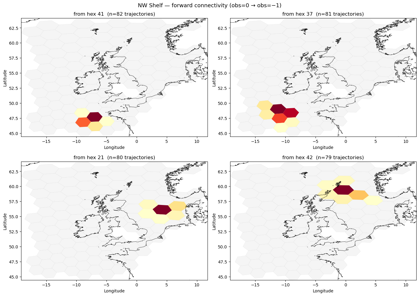
Forward connectivity heatmaps#

Pick four starting hexes that each launch the most trajectories — identified as the four from_id values with the highest marginal count. For each starting hex, plot the distribution of where its trajectories end up as a choropleth over the hex grid.

marginal = conn["count"].groupby(level="from_id").sum()
top4 = marginal.drop(index=INVALID_HEX_ID, errors="ignore").nlargest(4).index.tolist()

fig, axes = plt.subplots(2, 2, figsize=(14, 10))

for ax, from_hex in zip(axes.flat, top4):
    dest = conn.loc[(from_hex, slice(None))]
    dest = dest[dest.index != INVALID_HEX_ID]
    dest_gdf = gpd.GeoDataFrame(
        dest[["count"]].join(counts_valid[["geometry"]], how="left"),
        geometry="geometry",
        crs="EPSG:4326",
    ).dropna(subset=["geometry"])

    counts_valid.plot(ax=ax, color="whitesmoke", edgecolor="lightgrey", linewidth=0.2)
    dest_gdf.plot(column="count", ax=ax, cmap="YlOrRd", edgecolor="none", legend=False)
    coastlines.plot(ax=ax, color="black", linewidth=0.5)
    ax.set_xlim(counts_valid.total_bounds[[0, 2]])
    ax.set_ylim(counts_valid.total_bounds[[1, 3]])
    ax.set_title(f"from hex {from_hex}  (n={int(marginal[from_hex])} trajectories)")
    ax.set_xlabel("Longitude")
    ax.set_ylabel("Latitude")

fig.suptitle("NW Shelf — forward connectivity (obs=0 → obs=−1)", fontsize=13)
plt.tight_layout()
plt.show()

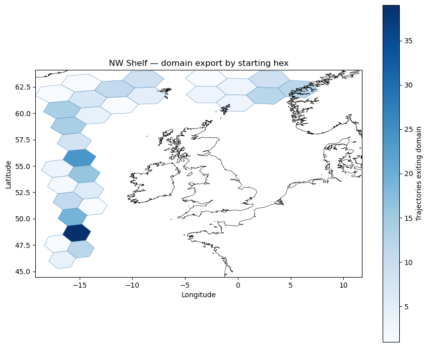
../_images/8670a09688b5be94d35c23f3479a7ea6c5efed461dd06a3f2274194d8e1d1057.png

INVALID_HEX_ID as a domain-exit signal#

In a well-run simulation, a particle becomes invalid when it exits the region covered by the circulation data — its lon/lat is set to NaN by the advection code. The connectivity entry (h, INVALID_HEX_ID) therefore records domain export: how many trajectories that started in hex $h$ eventually left the simulation area.

Filter the connectivity matrix to isolate these domain-exit pairs and inspect which starting hexes contribute most particles to the out-of-domain bucket.

domain_exits = conn.xs(INVALID_HEX_ID, level="to_id")
domain_exits_sorted = domain_exits.sort_values("count", ascending=False)
print(f"Hex cells that export particles out of domain: {len(domain_exits_sorted)}")
domain_exits_sorted.head(10)[["count"]]

Hex cells that export particles out of domain: 30

	count
from_id
66	39.0
161	24.0
93	19.0
126	16.0
290	14.0
243	14.0
79	12.0
86	12.0
113	12.0
204	11.0

Map the domain-exit counts as a heatmap. After .xs() the index is from_id (source hex), but the geometry column still contains None (it was a LineString to INVALID_HEX_ID). Re-attach hex polygon geometries by joining on the source hex ID before plotting. Darker hexes are the primary source regions for particles that leave the NW Shelf simulation domain.

exit_gdf = gpd.GeoDataFrame(
    domain_exits_sorted[["count"]].join(counts[["geometry"]], how="left"),
    geometry="geometry",
    crs="EPSG:4326",
).dropna(subset=["geometry"])

fig, ax = plt.subplots(figsize=(9, 7))
exit_gdf.plot(
    column="count",
    ax=ax,
    legend=True,
    legend_kwds={"label": "Trajectories exiting domain", "orientation": "vertical"},
    cmap="Blues",
    edgecolor="steelblue",
    linewidth=0.4,
)
coastlines.plot(ax=ax, color="black", linewidth=0.5)
ax.set_xlim(counts_valid.total_bounds[[0, 2]])
ax.set_ylim(counts_valid.total_bounds[[1, 3]])
ax.set_title("NW Shelf — domain export by starting hex")
ax.set_xlabel("Longitude")
ax.set_ylabel("Latitude")
plt.tight_layout()
plt.show()

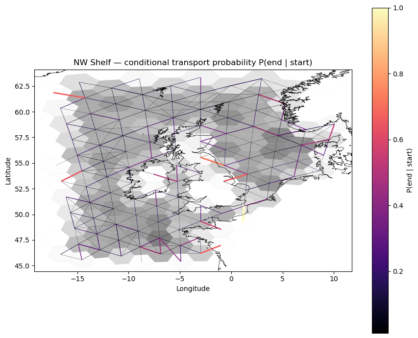
../_images/219f73ad08ee5b9458002358f75a6971e22bb94ca24d1e4683de803a511814df.png

Normalisation: conditional transport probability#

The raw connectivity $C(h_0, h_1)$ is a joint count. Dividing by the total number of trajectories that started in each hex $h_0$ gives the conditional probability of reaching destination $h_1$:

$$P(\text{end} = h_1 \mid \text{start} = h_0) = \frac{C(h_0, h_1)}{\displaystyle\sum_{h_1’} C(h_0, h_1’)}.$$

The denominator is the marginal count of all trajectories starting in $h_0$ — including those that exited the domain (counted in the INVALID_HEX_ID bucket). This ensures that probabilities sum to exactly 1 for every starting hex, with no information discarded.

Compute the marginal counts by summing over to_id within each from_id group, then divide.

marginal = conn["count"].groupby(level="from_id").transform("sum")
conn["prob"] = conn["count"] / marginal

Verify that the conditional probabilities sum to 1 for each starting hex (up to floating-point rounding).

prob_sums = conn["prob"].groupby(level="from_id").sum()
print("Min probability sum:", prob_sums.min())
print("Max probability sum:", prob_sums.max())

Min probability sum: 0.9999999999999999
Max probability sum: 1.0

Plot the in-domain conditional transport probability. Thicker, brighter edges indicate more probable connections. Only pairs where both endpoints are in-domain are shown.

conn_prob_valid = conn[conn.geometry.notna()]

fig, ax = plt.subplots(figsize=(9, 7))

counts_valid.plot(
    column="count",
    ax=ax,
    cmap="Greys",
    edgecolor="lightgrey",
    linewidth=0.2,
    alpha=0.5,
    legend=False,
)

max_prob = conn_prob_valid["prob"].max()
conn_prob_valid.plot(
    column="prob",
    ax=ax,
    cmap="magma",
    linewidth=(conn_prob_valid["prob"] / max_prob * 3).clip(lower=0.2),
    legend=True,
    legend_kwds={"label": "P(end | start)", "orientation": "vertical"},
)

coastlines.plot(ax=ax, color="black", linewidth=0.5)
ax.set_xlim(counts_valid.total_bounds[[0, 2]])
ax.set_ylim(counts_valid.total_bounds[[1, 3]])
ax.set_title("NW Shelf — conditional transport probability P(end | start)")
ax.set_xlabel("Longitude")
ax.set_ylabel("Latitude")
plt.tight_layout()
plt.show()

../_images/9f4d092e1a0c2d3b974cc234b3e35da215c12561007a205cfffd42241dbd8c35.png

Multi-generation connectivity: `hex_connectivity_power`#

The conn GeoDataFrame built above represents one generation of drift: each row encodes how many trajectories moved from a starting hex to an ending hex over a single observation period.

Raising this connectivity to the power $n$ asks: if the same drift pattern repeated itself $n$ times, where would a particle released from hex $h_i$ end up? Formally, the $n$-generation transfer matrix $T^{(n)}$ is defined by

$$T^{(n)}{ij} = (T^n){ij} = P!\bigl(\text{arrive at } h_j \text{ after } n \text{ generations} \mid \text{depart from } h_i\bigr),$$

where $T_{ij}$ is first obtained by row-normalising the raw counts $C(h_i, h_j)$.

INVALID_HEX_ID acts as an absorbing state by default: once a particle leaves the domain it stays out, so probability mass that flows into INVALID accumulates there over successive generations. Passing condition_on_valid=True instead zeros the INVALID column and renormalises, giving the conditional distribution over in-domain destinations for particles that remain in the domain for all $n$ steps.

from hextraj import hex_connectivity_power

conn2 = hex_connectivity_power(conn, n=2, hp=hp)
conn4 = hex_connectivity_power(conn, n=4, hp=hp)

Each row of the output should sum to 1: each starting hex’s probability mass is fully accounted for, either at a valid destination or at INVALID_HEX_ID.

prob_sums = conn2["probability"].groupby(level="from_id").sum()
print(prob_sums.describe())

count    116.000000
mean       0.999631
std        0.003979
min        0.957143
25%        1.000000
50%        1.000000
75%        1.000000
max        1.000000
Name: probability, dtype: float64

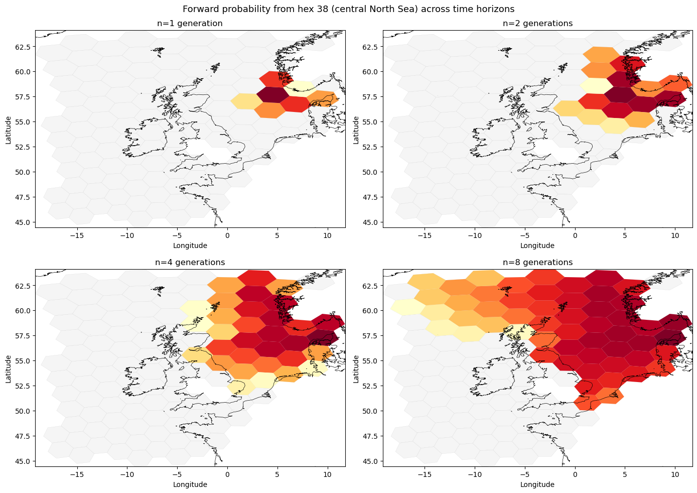
Forward probability maps across time horizons#

The four panels below show where hex 38 (approximately 4°E, 57°N — central North Sea) sends its particles after 1, 2, 4, and 8 generations of the same drift pattern. As $n$ increases, probability spreads over a wider area and accumulates in INVALID_HEX_ID (not shown) for particles that have exited the domain.

conn8 = hex_connectivity_power(conn, n=8, hp=hp)

conn1_prob = conn.copy()
marginal_from = conn1_prob["count"].groupby(level="from_id").transform("sum")
conn1_prob["probability"] = conn1_prob["count"] / marginal_from

from matplotlib.colors import LogNorm

from_hex = 38

generations = [(1, conn1_prob), (2, conn2), (4, conn4), (8, conn8)]

fig, axes = plt.subplots(2, 2, figsize=(14, 10))

for ax, (n, conn_n) in zip(axes.flat, generations):
    dest = conn_n.loc[(from_hex, slice(None))]
    dest = dest[dest.index != INVALID_HEX_ID]
    dest_gdf = gpd.GeoDataFrame(
        dest[["probability"]].join(counts_valid[["geometry"]], how="left"),
        geometry="geometry",
        crs="EPSG:4326",
    ).dropna(subset=["geometry"])

    counts_valid.plot(ax=ax, color="whitesmoke", edgecolor="lightgrey", linewidth=0.2)
    if len(dest_gdf) > 0:
        vmin = dest_gdf["probability"][dest_gdf["probability"] > 0].min()
        vmax = dest_gdf["probability"].max()
        dest_gdf.plot(
            column="probability", ax=ax, cmap="YlOrRd", edgecolor="none",
            norm=LogNorm(vmin=vmin, vmax=vmax), legend=False,
        )
    coastlines.plot(ax=ax, color="black", linewidth=0.5)
    ax.set_xlim(counts_valid.total_bounds[[0, 2]])
    ax.set_ylim(counts_valid.total_bounds[[1, 3]])
    ax.set_title(f"n={n} generation{'s' if n > 1 else ''}")
    ax.set_xlabel("Longitude")
    ax.set_ylabel("Latitude")

fig.suptitle(f"Forward probability from hex {from_hex} (central North Sea) across time horizons", fontsize=13)
plt.tight_layout()
plt.show()

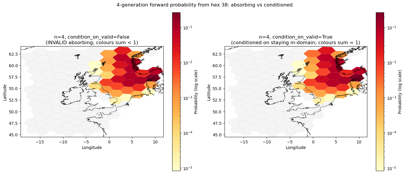
../_images/3f012b696a12223d09d8b4ce01662e461e2541c1be1bd5d5f738314381dfc172.png

Conditioning on staying in-domain: `condition_on_valid`#

The two panels below compare the 4-generation probability distribution for the same starting hex under the two INVALID treatments:

Left (condition_on_valid=False): INVALID is an absorbing state. Probability mass that has drained to INVALID is absent from the map — the hex colours show only the fraction of particles still in-domain, so the distribution sums to less than 1 over valid hexes.
Right (condition_on_valid=True): INVALID is removed before computing $T^4$, and each row is renormalised. The distribution conditions on the particle remaining in-domain for all 4 steps, so the colours sum to 1 over valid hexes. This reveals the relative spread among in-domain destinations independently of how many particles have left.

conn4_absorb = hex_connectivity_power(conn, n=4, hp=hp, condition_on_valid=False)
conn4_cond = hex_connectivity_power(conn, n=4, hp=hp, condition_on_valid=True)

fig, axes = plt.subplots(1, 2, figsize=(14, 6))

panels = [
    (conn4_absorb, "n=4, condition_on_valid=False\n(INVALID absorbing; colours sum < 1)"),
    (conn4_cond,   "n=4, condition_on_valid=True\n(conditioned on staying in-domain; colours sum = 1)"),
]

for ax, (conn_n, title) in zip(axes, panels):
    try:
        dest = conn_n.loc[(from_hex, slice(None))]
    except KeyError:
        dest = gpd.GeoDataFrame(columns=["probability", "geometry"])
        dest.index.names = ["to_id"]

    dest = dest[dest.index != INVALID_HEX_ID]
    dest_gdf = gpd.GeoDataFrame(
        dest[["probability"]].join(counts_valid[["geometry"]], how="left"),
        geometry="geometry",
        crs="EPSG:4326",
    ).dropna(subset=["geometry"])

    counts_valid.plot(ax=ax, color="whitesmoke", edgecolor="lightgrey", linewidth=0.2)
    if len(dest_gdf) > 0:
        vmin = dest_gdf["probability"][dest_gdf["probability"] > 0].min()
        vmax = dest_gdf["probability"].max()
        dest_gdf.plot(
            column="probability", ax=ax, cmap="YlOrRd", edgecolor="none",
            norm=LogNorm(vmin=vmin, vmax=vmax), legend=True,
            legend_kwds={"label": "Probability (log scale)", "orientation": "vertical"},
        )
    coastlines.plot(ax=ax, color="black", linewidth=0.5)
    ax.set_xlim(counts_valid.total_bounds[[0, 2]])
    ax.set_ylim(counts_valid.total_bounds[[1, 3]])
    ax.set_title(title)
    ax.set_xlabel("Longitude")
    ax.set_ylabel("Latitude")

fig.suptitle(f"4-generation forward probability from hex {from_hex}: absorbing vs conditioned", fontsize=12)
plt.tight_layout()
plt.show()

../_images/abfcadb446f103fa81211db8b8c2de49ad64280ad9d2edd5fb41deed008adb3f.png

Hex Analysis: Heatmaps and Connectivity

Contents

Hex Analysis: Heatmaps and Connectivity#

Setup#

Load the NW Shelf trajectory data#

Build a HexProj for the NW Shelf domain#

Hex heatmap: `hex_counts`#

Connectivity: `hex_connectivity`#

Forward connectivity heatmaps#

INVALID_HEX_ID as a domain-exit signal#

Normalisation: conditional transport probability#

Multi-generation connectivity: `hex_connectivity_power`#

Forward probability maps across time horizons#

Conditioning on staying in-domain: `condition_on_valid`#

Hex Analysis: Heatmaps and Connectivity

Contents

Hex Analysis: Heatmaps and Connectivity#

Setup#

Load the NW Shelf trajectory data#

Build a HexProj for the NW Shelf domain#

Hex heatmap: hex_counts#

Connectivity: hex_connectivity#

Forward connectivity heatmaps#

INVALID_HEX_ID as a domain-exit signal#

Normalisation: conditional transport probability#

Multi-generation connectivity: hex_connectivity_power#

Forward probability maps across time horizons#

Conditioning on staying in-domain: condition_on_valid#

Hex heatmap: `hex_counts`#

Connectivity: `hex_connectivity`#

Multi-generation connectivity: `hex_connectivity_power`#

Conditioning on staying in-domain: `condition_on_valid`#