Hex connectivity — NW Shelf trajectories#

Load the bundled NW Shelf trajectory dataset, label positions with hp.label(), and compute an origin–destination connectivity matrix using an efficient pandas groupby. Visualise as a choropleth + OD edge overlay.

Imports#

from importlib.resources import files
import numpy as np
import pandas as pd
import xarray as xr
import geopandas as gpd
from shapely.geometry import Polygon
from matplotlib import pyplot as plt
from hextraj import HexProj
from hextraj.hex_id import INVALID_HEX_ID

Set up HexProj#

We centre the projection on the data domain and use a fixed hex size of 50 km. With a flat-top orientation, the meridional extent of one hex is $\sqrt{3} \times$ hex_size_meters ≈ 87 km.

lon_origin = float((ds.lon.min() + ds.lon.max()) / 2)
lat_origin = float((ds.lat.min() + ds.lat.max()) / 2)
hp = HexProj(lon_origin=lon_origin, lat_origin=lat_origin, hex_size_meters=50_000)
hp

HexProj(projection_name='laea', lon_origin=-2.9847207069396973, lat_origin=54.370880126953125, hex_size_meters=50000, hex_orientation='flat', )

Label all positions#

hp.label() maps every (lon, lat) pair to a single int64 hex ID via a Cantor-encoded (q, r) axial coordinate. NaN positions (beached or exited particles) are assigned INVALID_HEX_ID rather than raising.

hex_ids = hp.label(ds.lon.values, ds.lat.values)  # shape (5000, 20)
print(f"hex_ids shape: {hex_ids.shape}, dtype: {hex_ids.dtype}")
print(f"unique hexes: {len(np.unique(hex_ids[hex_ids != INVALID_HEX_ID]))}")

hex_ids shape: (2500, 20), dtype: int64
unique hexes: 391

Dask recipe for larger-than-memory arrays#

hp.label() materialises at the pyproj boundary, so all input arrays must fit in memory at once. For larger-than-memory arrays, wrap hp.label() in dask.array.map_blocks():

import dask.array as da
lon_dask = da.from_array(ds.lon.values, chunks=(1000, 20))
lat_dask = da.from_array(ds.lat.values, chunks=(1000, 20))
hex_ids_lazy = da.map_blocks(hp.label, lon_dask, lat_dask, dtype=np.int64)
hex_ids = hex_ids_lazy.compute()

Each chunk is labelled independently, keeping peak memory proportional to chunk size.

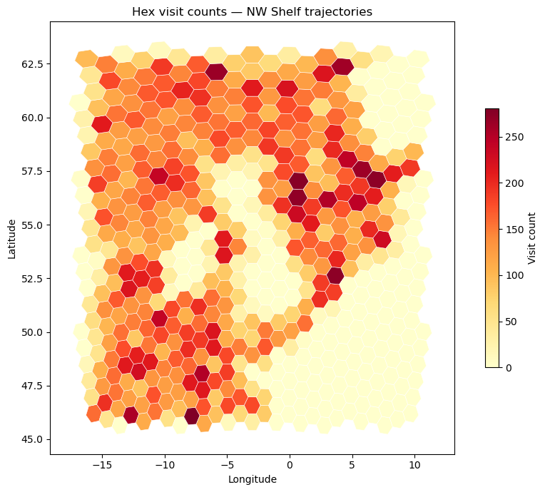
Visit heatmap#

Count how many trajectory positions land in each hex cell, then visualise as a choropleth over the full domain. This reveals the dominant flow corridors regardless of trajectory direction.

counts = pd.Series(hex_ids.ravel()).value_counts()
counts = counts.drop(INVALID_HEX_ID, errors="ignore")
print(f"{len(counts)} hexes visited, max {counts.max()} visits")

391 hexes visited, max 281 visits

region_polygon = Polygon([
    (ds.lon.min(), ds.lat.min()),
    (ds.lon.max(), ds.lat.min()),
    (ds.lon.max(), ds.lat.max()),
    (ds.lon.min(), ds.lat.max()),
    (ds.lon.min(), ds.lat.min()),
])
region_gdf = hp.to_geodataframe(hp.region_of_hexes(region_polygon))
region_gdf["count"] = counts.reindex(region_gdf.index).fillna(0).astype(int)
print(f"{len(region_gdf)} hexes in region")

537 hexes in region

ax = region_gdf.plot(
    column="count", cmap="YlOrRd", edgecolor="white", linewidth=0.4,
    figsize=(9, 7), legend=True, legend_kwds={"label": "Visit count", "shrink": 0.6},
)
ax.set_title("Hex visit counts — NW Shelf trajectories")
ax.set_xlabel("Longitude"); ax.set_ylabel("Latitude")
plt.tight_layout()

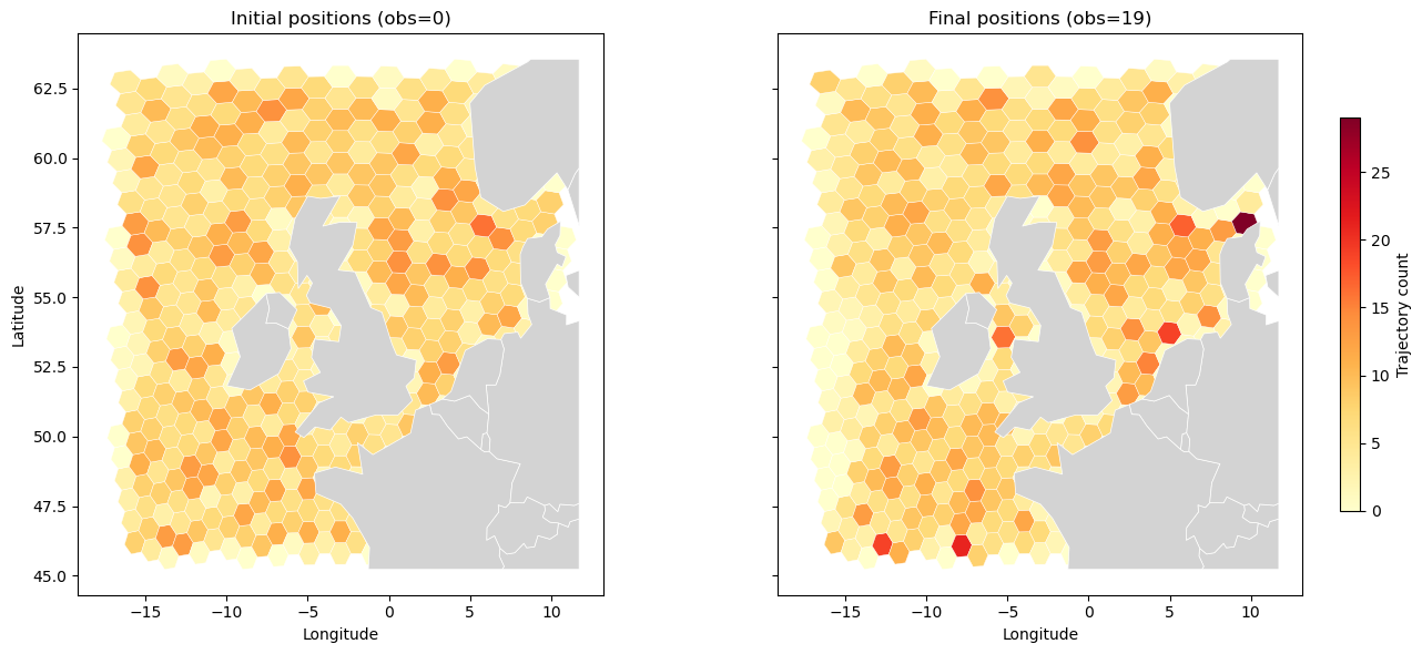
../_images/080d6a32ae074a0ad18b6fa920d2d50b082773a82607fd8890ffb6b184d5a2bf.png

Initial and final position heatmaps#

Comparing where trajectories start (obs=0) and end (obs=19) reveals net displacement — areas of convergence appear as hotspots in the final map that have no corresponding source in the initial map.

world = gpd.read_file(
    "https://naciscdn.org/naturalearth/110m/cultural/ne_110m_admin_0_countries.zip"
)

counts_initial = pd.Series(hp.label(ds.lon.values[:, 0],  ds.lat.values[:, 0])).value_counts()
counts_final   = pd.Series(hp.label(ds.lon.values[:, -1], ds.lat.values[:, -1])).value_counts()
for c in (counts_initial, counts_final):
    c.drop(INVALID_HEX_ID, errors="ignore", inplace=True)

region_gdf["count_initial"] = counts_initial.reindex(region_gdf.index).fillna(0).astype(int)
region_gdf["count_final"]   = counts_final.reindex(region_gdf.index).fillna(0).astype(int)

vmax = max(region_gdf["count_initial"].max(), region_gdf["count_final"].max())

fig, axes = plt.subplots(1, 2, figsize=(14, 6), sharey=True)
for ax, col, title in zip(axes, ["count_initial", "count_final"], ["Initial positions (obs=0)", "Final positions (obs=19)"]):
    region_gdf.plot(column=col, cmap="YlOrRd", edgecolor="white", linewidth=0.3,
                    vmin=0, vmax=vmax, ax=ax, legend=(ax is axes[1]),
                    legend_kwds={"label": "Trajectory count", "shrink": 0.7})
    world.clip(region_gdf.total_bounds).plot(ax=ax, color="lightgray", edgecolor="white", linewidth=0.5)
    ax.set_title(title)
    ax.set_xlabel("Longitude")
axes[0].set_ylabel("Latitude")
plt.tight_layout()

../_images/5e181ca2df3177f5fbec24a6199b38a925ca3bd12aeae213b28fe12cc59f3677.png

OD connectivity — efficient recipe#

We want to count how many trajectories connect each origin hex to each destination hex. The naive approach — a boolean broadcast over all trajectories and all hex pairs — scales as $O(N_{\text{traj}} \times N_{\text{hex}}^2)$ and quickly becomes impractical.

Instead we extract just the first and last observed hex ID for every trajectory, build a MultiIndex, and delegate counting to pandas.Series.groupby. This is $O(N_{\text{traj}} \log N_{\text{traj}})$ and allocates no intermediate matrix.

from_ids = hp.label(ds.lon.values[:, 0],  ds.lat.values[:, 0])
to_ids   = hp.label(ds.lon.values[:, -1], ds.lat.values[:, -1])
valid = (from_ids != INVALID_HEX_ID) & (to_ids != INVALID_HEX_ID)
from_ids, to_ids = from_ids[valid], to_ids[valid]
print(f"{valid.sum()} valid trajectories out of {len(valid)}")

2367 valid trajectories out of 2500

idx = pd.MultiIndex.from_arrays([from_ids, to_ids], names=["from_id", "to_id"])
od_counts = pd.Series(1, index=idx).groupby(level=[0, 1]).sum()
print(f"{len(od_counts)} unique OD pairs, max weight {od_counts.max()}")
od_counts.head()

1273 unique OD pairs, max weight 11

from_id  to_id
1        0        1
         1        2
2        0        1
         1        2
         32       1
dtype: int64

od_gdf = hp.edges_geodataframe(
    od_counts.index.get_level_values("from_id"),
    od_counts.index.get_level_values("to_id"),
    weight=od_counts.values,
)
print(f"OD GeoDataFrame: {od_gdf.shape}")
od_gdf.head()

OD GeoDataFrame: (1273, 2)

		weight	geometry
from_id	to_id
1	0	1	LINESTRING (-4.12785 53.97642, -2.98472 54.37088)
1	1	2	LINESTRING (-4.12785 53.97642, -4.12785 53.97642)
2	0	1	LINESTRING (-2.98472 53.59281, -2.98472 54.37088)
	1	2	LINESTRING (-2.98472 53.59281, -4.12785 53.97642)
	32	1	LINESTRING (-2.98472 53.59281, -5.33649 55.12638)

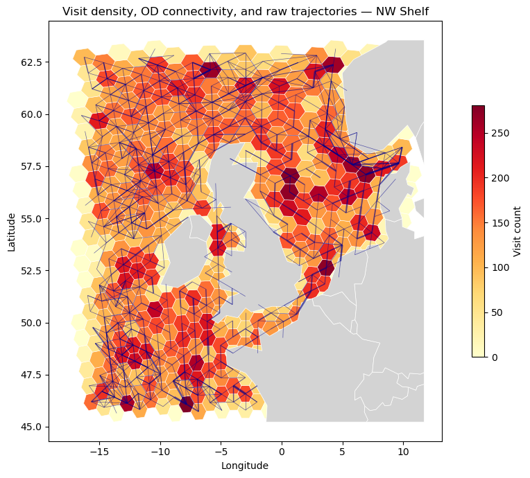
Combined plot#

Overlay the OD edge network on the visit choropleth. Edge width is scaled linearly to trajectory count, making high-traffic corridors immediately visible.

ax = region_gdf.plot(
    column="count", cmap="YlOrRd", edgecolor="white", linewidth=0.4,
    figsize=(9, 7), legend=True, legend_kwds={"label": "Visit count", "shrink": 0.6},
)
world.clip(region_gdf.total_bounds).plot(ax=ax, color="lightgray", edgecolor="white", linewidth=0.5)
w = od_gdf["weight"]
od_gdf.plot(
    ax=ax,
    linewidth=0.5 + 3.0 * (w - w.min()) / (w.max() - w.min() + 1),
    color="darkblue", alpha=0.6,
)
ax.set_title("Visit density, OD connectivity, and raw trajectories — NW Shelf")
ax.set_xlabel("Longitude"); ax.set_ylabel("Latitude")
plt.tight_layout()

../_images/5bee256b1709d7bdcc2144a0f7a3e6f54a9d1e0c2f6df862ccba8eb379adbad4.png

Hex connectivity — NW Shelf trajectories

Contents